Regression Analysis
Regression analysis is used to model the relationship between a response variable and one or more predictor variables.
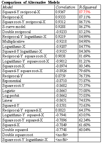
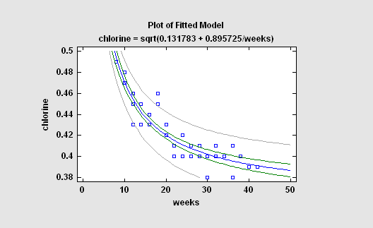
Simple Regression
The simplest regression models involve a single response variable Y and a single predictor variable X. Statgraphics will fit a variety of functional forms, listing the models in decreasing order of R-squared. If outliers are suspected, resistant methods can be used to fit the models instead of least squares.
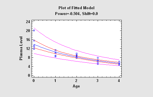
Box-Cox Transformations
When the response variable does not follow a normal distribution, it is sometimes possible to use the methods of Box and Cox to find a transformation that improves the fit. Their transformations are based on powers of Y. Statgraphics will automatically determine the optimal power and fit an appropriate model.
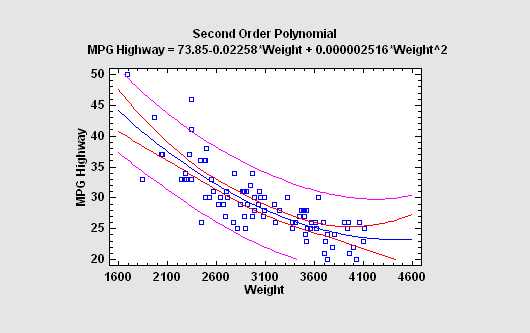
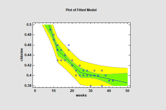
Polynomial Regression
Another approach to fitting a nonlinear equation is to consider polynomial functions of X. For interpolative purposes, polynomials have the attractive property of being able to approximate many kinds of functions.
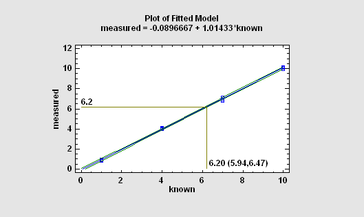
Calibration Models
In a typical calibration problem, a number of known samples are measured and an equation is fit relating the measurements to the reference values. The fitted equation is then used to predict the value of an unknown sample by generating an inverse prediction (predicting X from Y) after measuring the sample.
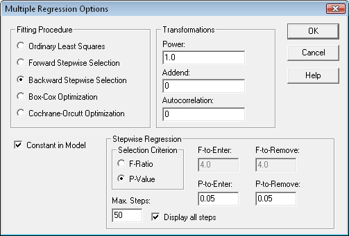
Multiple Regression
The Multiple Regression procedure fits a model relating a response variable Y to multiple predictor variables X1, X2, ... . The user may include all predictor variables in the fit or ask the program to use a stepwise regression to select a subset containing only significant predictors. At the same time, the Box-Cox method can be used to deal with non-normality and the Cochrane-Orcutt procedure to deal with autocorrelated residuals.
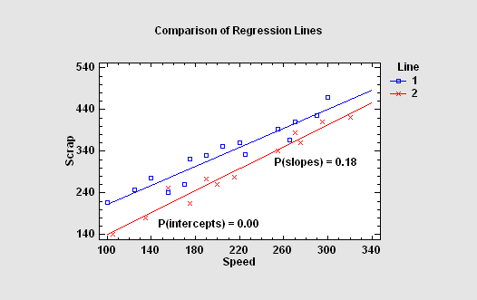
Comparison of Regression Lines
In some situations, it is necessary to compare several regression lines. Statgraphics will fit parallel or non-parallel linear regressions for each level of a "BY" variable and perform statistical tests to determine whether the intercepts and/or slopes of the lines are significantly different.
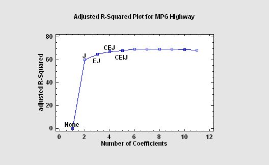
Regression Model Selection
If the number of predictors is not excessive, it is possible to fit regression models involving all combinations of 1 predictor, 2 predictors, 3 predictors, etc., and sort the models according to a goodness-of fit statistic. In Statgraphics, the Regression Model Selection procedure implements such a scheme, selecting the models which give the best values of the adjusted R-Squared or of Mallows' Cp statistic.
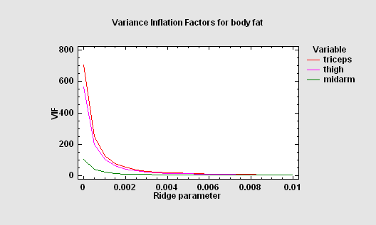
Ridge Regression
When the predictor variables are highly correlated amongst themselves, the coefficients of the resulting least squares fit may be very imprecise. By allowing a small amount of bias in the estimates, more reasonable coefficients may often be obtained. Ridge regression is one method to address these issues. Often, small amounts of bias lead to dramatic reductions in the variance of the estimated model coefficients.
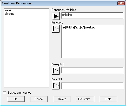
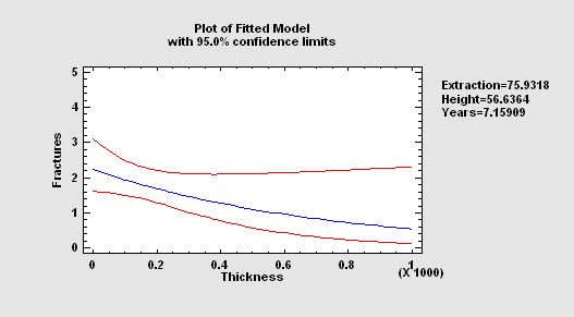
Nonlinear Regression
Most least squares regression programs are designed to fit models that are linear in the coefficients. When the analyst wishes to fit an intrinsically nonlinear model, a numerical procedure must be used. The Statgraphics Nonlinear Least Squares procedure uses an algorithm due to Marquardt to fit any function entered by the user.
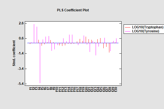
Partial Least Squares
Partial Least Squares is designed to construct a statistical model relating multiple independent variables X to multiple dependent variables Y. The procedure is most helpful when there are many predictors and the primary goal of the analysis is prediction of the response variables. Unlike other regression procedures, estimates can be derived even in the case where the number of predictor variables outnumbers the observations. PLS is widely used by chemical engineers and chemometricians for spectrometric calibration.
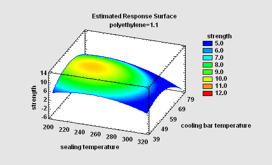
General Linear Models
The GLM procedure is useful when the predictors include both quantitative and categorical factors. When fitting a regression model, it provides the ability to create surface and contour plots easily.
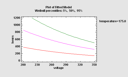
Life Data Regression
To describe the impact of external variables on failure times, regression models may be fit. Unfortunately, standard least squares techniques do not work well for two reasons: the data are often censored, and the failure time distribution is rarely Gaussian. For this reason, Statgraphics and Minitab both provide a special procedure that will fit life data regression models with censoring, assuming either an exponential, extreme value, logistic, loglogistic, lognormal, normal or Weibull distribution.
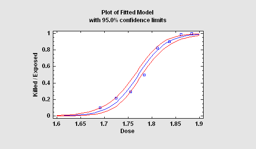
Regression Analysis for Proportions
When the response variable is a proportion or a binary value (0 or 1), standard regression techniques must be modified. There are two important procedures for this situation: Logistic Regression and Probit Analysis. Both methods yield a prediction equation that is constrained to lie between 0 and 1.
Regression Analysis for Counts
For response variables that are counts, Statgraphics provides two procedures: a Poisson Regression and a Negative Binomial Regression. Each fits a loglinear model involving both quantitative and categorical predictors.
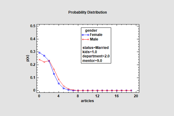
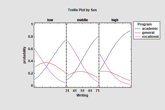
Multinomial Logistic Regression
The Multinomial Logistic Regression procedure fits regression models to describe the relationship between a categorical dependent variable Y and one or more independent variables. The independent variables may be either quantitative or categorical. Unlike original regression in which the set of values for the dependent variable has a meaningful order, the order of values for Y has no effect on the fitted models.
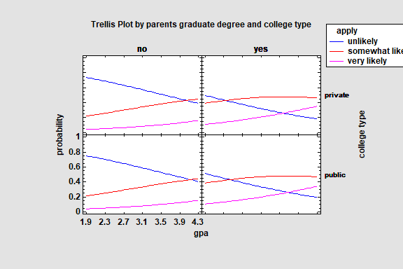
Ordinal Regression
The Ordinal Regression procedure fits regression models to describe the relationship between an ordinal dependent variable Y and one or more independent variables. The independent variables may be either quantitative or categorical. Ordinal variables contain a discrete set of values that have a meaningful order. For example, the response to a survey question might contain one of the values strongly disagree, disagree, no opinion, agree or strongly agree. Given various characteristics of the responder such as age, gender and yearly income, an ordinal regression model could estimate the probabilities that a responder would answer the question in each of the 5 ways.
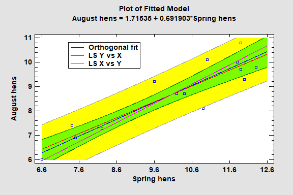
The Orthogonal Regression procedure is designed to construct a statistical model describing the impact of a single quantitative factor X on a dependent variable Y, when both X and Y are observed with error. Any of 27 linear and nonlinear models may be fit. Tests are run to determine the statistical significance of the model. The fitted model may be plotted with confidence limits and/or prediction limits. Residuals may also be plotted and unusual observations identified.
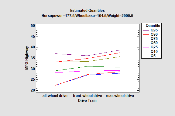
The Quantile Regression procedure fits linear models to describe the relationship between selected quantiles of a dependent variable Y and one or more independent variables. The independent variables may be either quantitative or categorical. Unlike standard multiple regression procedures in which the model is used to predict mean response, quantile regression models may be used to predict any percentile. Median regression is a special case where the quantile to be predicted is the 50th percentile.
Piecewise Linear Regression
The Piecewise Linear Regression procedure is designed to fit a regression model where the relationship between the dependent variable Y and the independent variable X is a continuous function consisting of 2 or more linear segments. The function is estimated using nonlinear least squares. The user specifies the number of segments and initial estimates of the locations where the segments join.
Zero-Inflated Poisson Regression
The Zero Inflated Count Regression procedure is designed to fit a regression model in which the dependent variable Y consists of counts. The fitted regression model relates Y to one or more predictor variables X, which may be either quantitative or categorical. It is similar to the procedures for Poisson Regression and Negative Binomial Regression except that it contains an additional component that represents the occurrence of more zeroes than would be expected in those models. Data containing excess zeroes is very common, including such diverse examples as the number of days a student is absent from school, the number of insurance claims within a population where not everyone has insurance, the number of defects in a manufactured item, and wild animal counts.