Multivariate Methods
Multivariate statistical methods are used to analyze the joint behavior of more than one random variable. There are a wide range of multivariate techniques available, as may be seen from the examples below.
| Methodology |
| Cluster Analysis |
| Discriminant Analysis |
| Matrix Plot |
| Multidimensional Scaling |
| Neural Network Analysis |
| Partial Least Squares |
| Principal Components and Factor Analysis |
| Radar/Spider Plot |
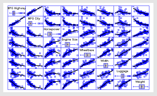
Matrix Plot
Matrix plots are used to display all pairs of X-Y plots for a set of quantitative variables. They are a good method for detecting pairs of variables that are strongly correlated. It is also possible to detect cases that appear to be outliers. The matrix plot above has two additions:
1. A box-and-whisker plot for each variable in the diagonal locations.
2. A robust LOWESS smooth for each plot, which highlights the estimated relationships between the variables.
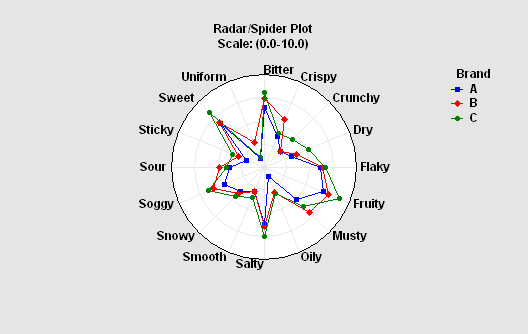
Radar/Spider Plot
A radar or spider plot is used to display the values of several quantitative variables on a case-by-case basis. The plot at the left compares characteristics of 3 different brands.
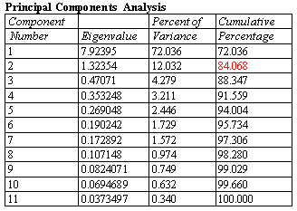
Principal Components and Factor Analysis
A principal components or factor analysis derives linear combinations of multiple quantitative variables that explain the largest percentage of the variation amongst those variables. These types of analyses are used to reduce the dimensionality of the problem in order to better understand the underlying factors affecting those variables. In many cases, a small number of components may explain a large percentage of the overall variability. Proper interpretation of the factors can provide important insights into the mechanisms that are at work.
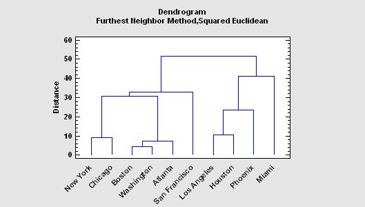
Cluster Analysis
A cluster analysis groups observations or variables based on similarities between them. The dendrogram at the left shows the results of hierarchical clustering procedure, which begins with separate observations and groups them together based upon the distance between them in a multivariate space.
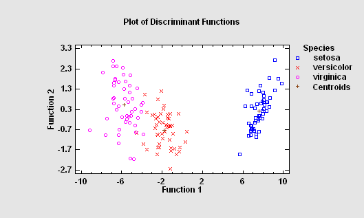
Discriminant Analysis
The Discriminant Analysis procedure is designed to help distinguish between two or more groups of data based on a set of p observed quantitative variables. It does so by constructing discriminant functions that are linear combinations of the variables. The objective of such an analysis is usually one or both of the following:
1. to be able to describe observed cases mathematically in a manner that separates them into groups as well as possible.
2. to be able to classify new observations as belonging to one or another of the groups.
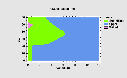
Neural Network Classifier
The Neural Network Classifier implements a nonparametric method for classifying observations into one of g groups based on p observed quantitative variables. Rather than making any assumption about the nature of the distribution of the variables within each group, it constructs a nonparametric estimate of each group’s density function at a desired location based on neighboring observations from that group. The estimate is constructed using a Parzen window that weights observations from each group according to their distance from the specified location.
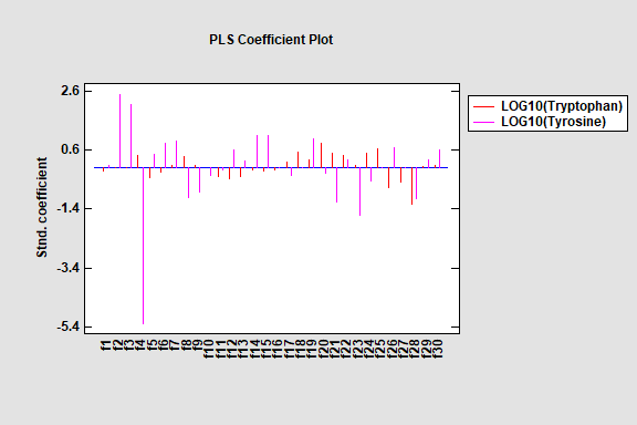
Partial Least Squares
Partial Least Squares is designed to construct a statistical model relating multiple independent variables X to multiple dependent variables Y. The procedure is most helpful when there are many predictors and the primary goal of the analysis is prediction of the response variables. Unlike other regression procedures, estimates can be derived even in the case where the number of predictor variables outnumbers the observations. PLS is widely used by chemical engineers and chemometricians for spectrometric calibration.
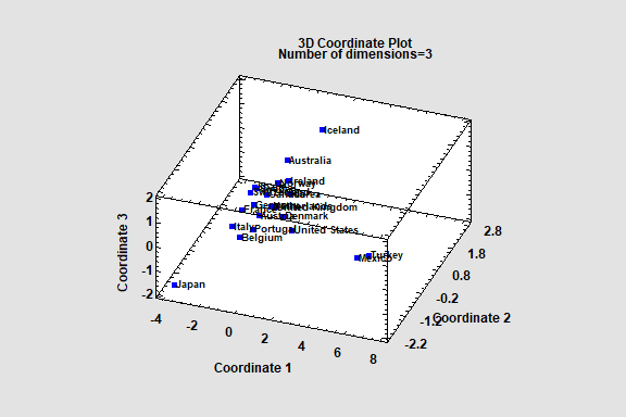
Multidimensional Scaling
dimensional space. Given an n by n matrix of distances between each pair of n multivariate observations, the procedure searches for a low-dimensional representation of those observations that preserves the distances between them as well as possible. The primary output is a map of the points in that low-dimensional space (usually 2 or 3 dimensions).
Input to the procedure may be either:
1. An n by n matrix of distances or “dissimilarities”.
2. An n by p matrix of observations for p variables, from which a distance matrix may be constructed.