Probability Distributions
Statistical software programs contain various procedures for manipulating probability distributions. Each of a selected set of distributions may be plotted, fit to data, and used to calculate critical values or tail areas. Random samples may also be generated from each of the distributions.
Probability Distributions
The Statgraphics Probability Distributions procedure calculates probabilities for 46 discrete and continuous distributions. It will plot the probability density or mass function, cumulative distribution function, survivor function, log survivor function, or hazard function. It also calculates critical values and tail areas. Random samples may be generated from any of the distributions given specified parameters value.
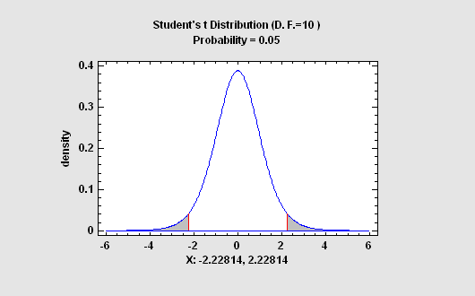
Sampling Distributions
The Sampling Distributions procedure calculates tail areas and critical values for the normal, Student's t, chi-square, and F distributions. It also plots the calculated results.
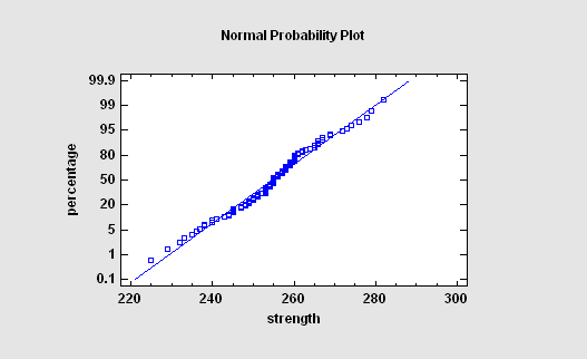
Normal Probability Plot
The Normal Probability Plot is used to help judge whether or not a sample of numeric data comes from a normal distribution. If it does, the points should fall close to a straight line when plotted against the specially scaled Y-axis. For non-normal data, you can often determine the type of departure from normality by examining the way in which the data deviate from the normal reference line.
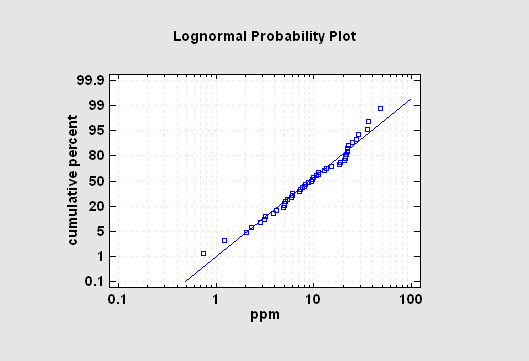
Probability Plots for Nonnormal Data
The Distribution Fitting (Uncensored Data) procedure fits any of 46 probability distributions to a column of numeric data. The data are assumed to be uncensored, i.e., the data represent random samples from the selected distribution. If requested, many distributions may be fit and ordered by their ability to match the data. Goodness-of-fit tests are performed to determine which distributions adequately model the observed values.
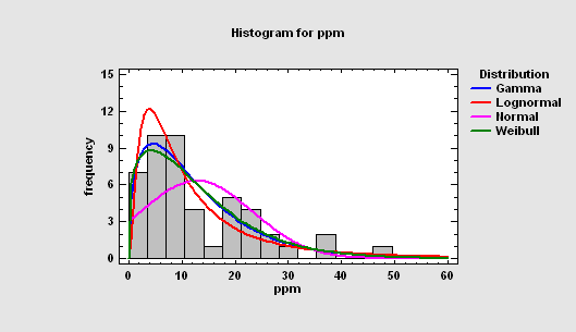
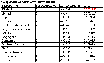
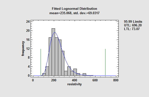
Distribution Fitting (Uncensored Data)
The Distribution Fitting (Uncensored Data) procedure fits any of 46 probability distributions to a column of numeric data. The data are assumed to be uncensored, i.e., the data represent random samples from the selected distribution. If requested, many distributions may be fit and ordered by their ability to match the data. Goodness-of-fit tests are performed to determine which distributions adequately model the observed values.
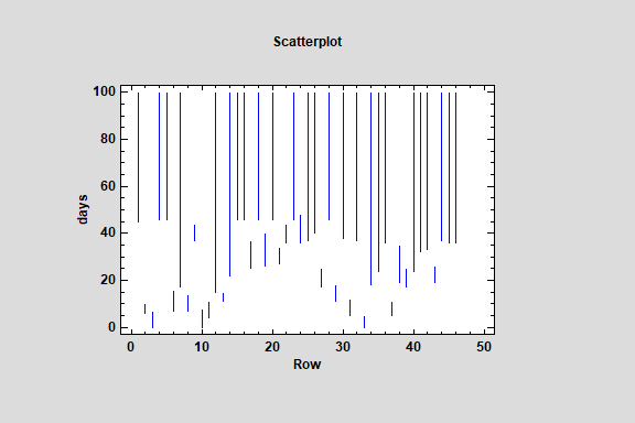
Distribution Fitting (Censored Data)
The Distribution Fitting (Censored Data) procedure fits any of 45 probability distributions to a column of censored numeric data. Censoring occurs when some of the data values are not known exactly. For example, when measuring failure times, some items under study may not have failed when the study is stopped, resulting in only a lower bound on the failure times for those items. As with uncensored data, the distributions may be sorted according to their goodness-of-fit.
Distribution Fitting (Arbitrarily Censored Data)
The Distribution Fitting (Arbitrarily Censored Data) procedure analyzes data in which one or more observations are not known exactly. Observations may be left-censored, right-censored, or interval-censored. The procedure calculates summary statistics, fits distributions, creates graphs, and calculates a nonparametric estimate of the survival function.
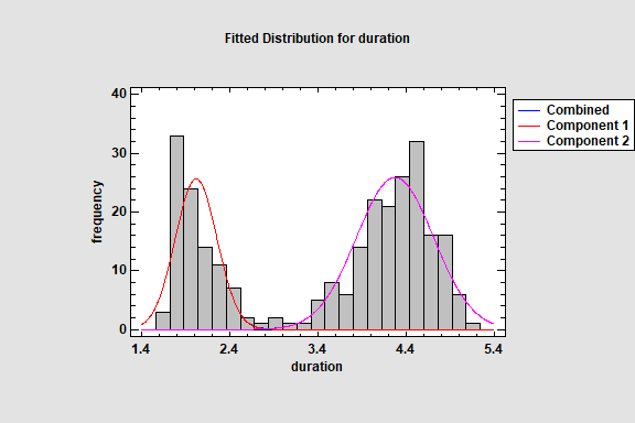
Distribution Fitting (Univariate Mixture Distributions)
The Distribution Fitting (Univariate Mixture Models) fits a distribution to continuous numeric data that consists of a mixture of 2 or more univariate Gaussian distributions. The components of the mixture may represent different groups in the sample used to fit the overall distribution, or the mixture model may approximate some distribution with a complicated shape. The procedure fits the distribution, creates graphs, and calculates tail areas and critical values. Tools are also provided for determining how many components are needed to represent a data sample.
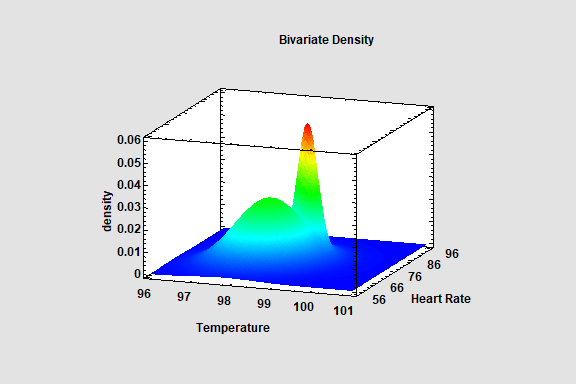
Distribution Fitting (Bivariate Mixture Distributions)
The Distribution Fitting (Univariate Mixture Models) fits a distribution to continuous numeric data that consists of a mixture of 2 or more univariate Gaussian distributions. The components of the mixture may represent different groups in the sample used to fit the overall distribution, or the mixture model may approximate some distribution with a complicated shape. The procedure fits the distribution, creates graphs, and calculates tail areas and critical values. Tools are also provided for determining how many components are needed to represent a data sample.
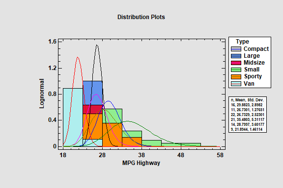
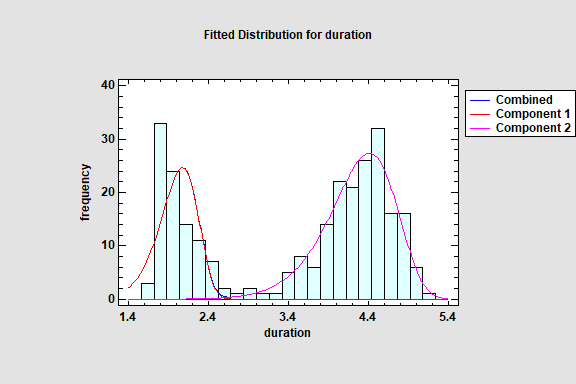
Distribution Fitting (Non-Normal Mixture Distributions)
The Distribution Fitting (Non-Normal Mixture Distributions) procedure fits a distribution to continuous numeric data that consist of a mixture of 2 or more univariate normal, Weibull, gamma or lognormal distributions. The components of the mixture may represent different groups in the sample used to fit the overall distribution, or the mixture model may approximate some distribution with a complicated shape.
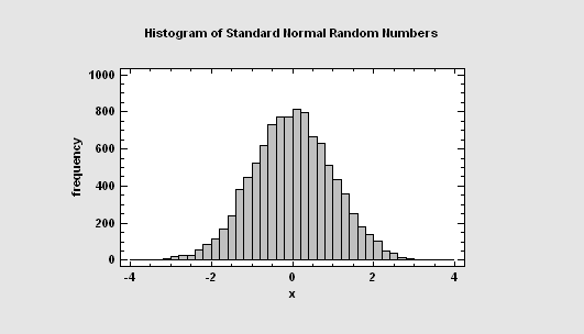
Random Number Generation
Random numbers may be generated from any of the 46 probability distributions using the Probability Distributions procedure. They may also be generated as part of the Monte Carlo simulations in Statgraphics Centurion.
Multivariate Normal Random Numbers
This procedure generates random numbers from a multivariate normal distribution involving up to 12 variables. The user inputs the variable means, standard deviations, and the correlation matrix. Random samples are generated which may be saved to the Statgraphics databook.
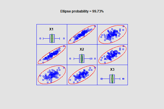
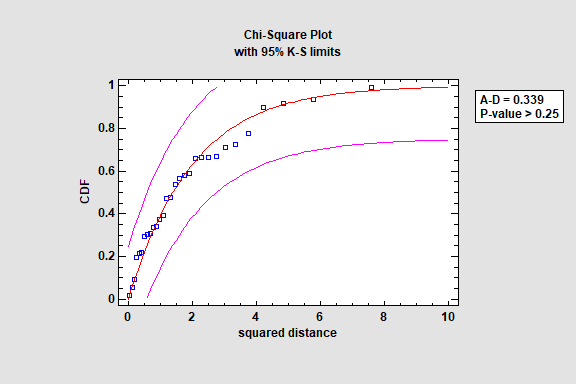
Multivariate Normality Test
This procedure tests whether a set of random variables could reasonably have come from a multivariate normal distribution. It includes Royston’s H test and tests based on a chi-square plot of the squared distances of each observation from the sample centroid.
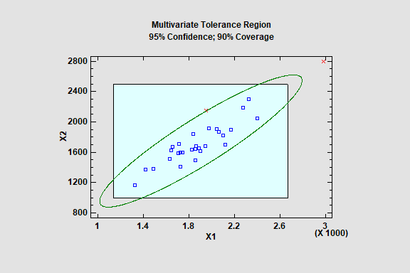
Statistical Tolerance Limits
Statistical tolerance limits give a range of values for a variable such that one may be 100(1-alpha)% confident that P percent of the population from which a data sample comes falls within that range. The limits may be based on a particular distribution such as the normal or Weibull distribution, or they may be constructed using a nonparametric approach.
The Multivariate Tolerance Limits procedure creates statistical tolerance limits for data consisting of more than one variable. It includes a tolerance region that bounds a selected p% of the population with 100(1-a)% confidence. It also includes joint simultaneous tolerance limits for each of the variables using a Bonferroni approach. The data are assumed to be a random sample from a multivariate normal distribution. Multivariate tolerance limits are often compared to specifications for multiple variables to determine whether or not most of the population is within spec.
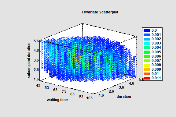
Trivariate Density Statlet
The Trivariate Density Statlet displays the estimated density function for 3 columns of numeric data. It does so using either a 3-dimensional contour plot or a 3-dimensional mesh plot. The joint distribution of the 3 variables may either be assumed to be multivariate normal or be estimated using a nonparametric approach.